Suliga Formulae
August 3, 2022
A Starting Note: I tried to make this page accessible for most viewing platforms. This being said, there are a lot of math equations/expressions here that may be difficult to see properly on larger screens. If this is the case for you, right click (hold down if using a tablet) on \(\textrm{this text}\) or any of the sections containing math-formatted text and a small MathJax menu will pop up. Click on “Math Settings” > “Scale All Math…” and input a number greater than 100 to increase the size of the math text. You can also set a zoom trigger to cause a bigger window containing the math section to pop up on a double click.
This post will showcase two different formulas that I came up with in my latter years of high school.
\[\int_{a}^{b} f(x) \space dx = \] \[b \times f(b) - a \times f(a) + \int_{f(b)}^{f(a)} f^{-1}(x) \space dx\]
The first is a very approachable idea, that can be understood without much knowledge of calculus. It stemmed from simply drawing shapes on a whiteboard in my bedroom, and came from an unawareness of previously-derived ways to integrate inverse trig functions. I didn’t know these existed so I came up with my own way to integrate a function in terms of its inverse.
\[\int_{-\infty}^{\infty}e^{ax^{2}+bx+c} \space dx = \] \[\lim_{n \to \infty} e^{c - \frac{b^{2}}{4a}}\sqrt{\frac{\pi}{a}(e^{an} - 1)}\]
The second, coined by my friends as The Suliga Theorem (which I very much disagree with this name, theorems are supposed to be useful), is a generalization of a discovery first popularized by and named after one of history’s smartest minds, Carl Friedrich Gauss. I hope this example sparks a wonder in you that it did me when I was first discovering this for myself. This concept assumes the reader is comfortable with single-variable integral calculus and using a polar representation of values.
Suliga Formula 1
\[\int_{a}^{b} f(x) \space dx = \] \[b \times f(b) - a \times f(a) + \int_{f(b)}^{f(a)} f^{-1}(x) \space dx\]
As I mentioned above, this formula originated from the question that I’m sure all students ask at some point - how can I integrate inverse trig functions? Formulas for such expressions do exist, but are super obscure, and I wasn’t aware of their existence. One can be seen below:
\[\int sec ^{-1} (x) \space dx = \] \[x \space sec^{-1}(x) - \text{ln}(x + \sqrt{x^{2} - 1}) + c\]
So, March 1, 2019, I brought out my trusty math whiteboard and started drawing shapes and came up with a seemingly working method to do this. Here are the original pictures I took to show to some of my math teachers to check. It pains me to look back on all of the excluded \(dx\)’s, so please excuse my junior-year math naivety.

Here I just started with an easy example. I had to create a function that was invertible and whose parts could be easily identified when looking at a diagram. I chose a simple linear function, \(f(x) = \frac{1}{2}x + 3\). In this instance this means \(f^{-1}(x) = 2x - 6\), check this for yourself. It’s also worth noting that somehow I managed to get the axis intercepts wrong when plotting these up, so that’s embarassing, however this doesn’t change the thinking.
This is a quick markup of my example, but it shows the idea behind what I was trying to accomplish very well. The “sections” of this graph which I shaded in different colors, are maintained throughout inversion, but are just shifted around. In fact, everything is reflected about the line \(y=x\), but that’s not too important here upfront.
I was able to derive a formula for the area that I wanted, which is in the dashed section in this diagram, but you’ll notice that this function still depends on integrating \(f(x)\), and the whole point of doing this was to bypass this and treat the integral of a function in terms of just the integral of its inverse.

With some tricky splitting apart of the original integral and applying what I had already found twice, such that the integral that still depended on \(f\) turned into an integral with bounds \(0 \to 0\), I was able to then reconstruct the integral parts again, I was able to get a final answer in terms of evaluating \(f\) at the original bounds and then integrating the inverse function.
Yes, looking back I see now that I could’ve gone right to this step from the beginning, but I didn’t realize this at the time.
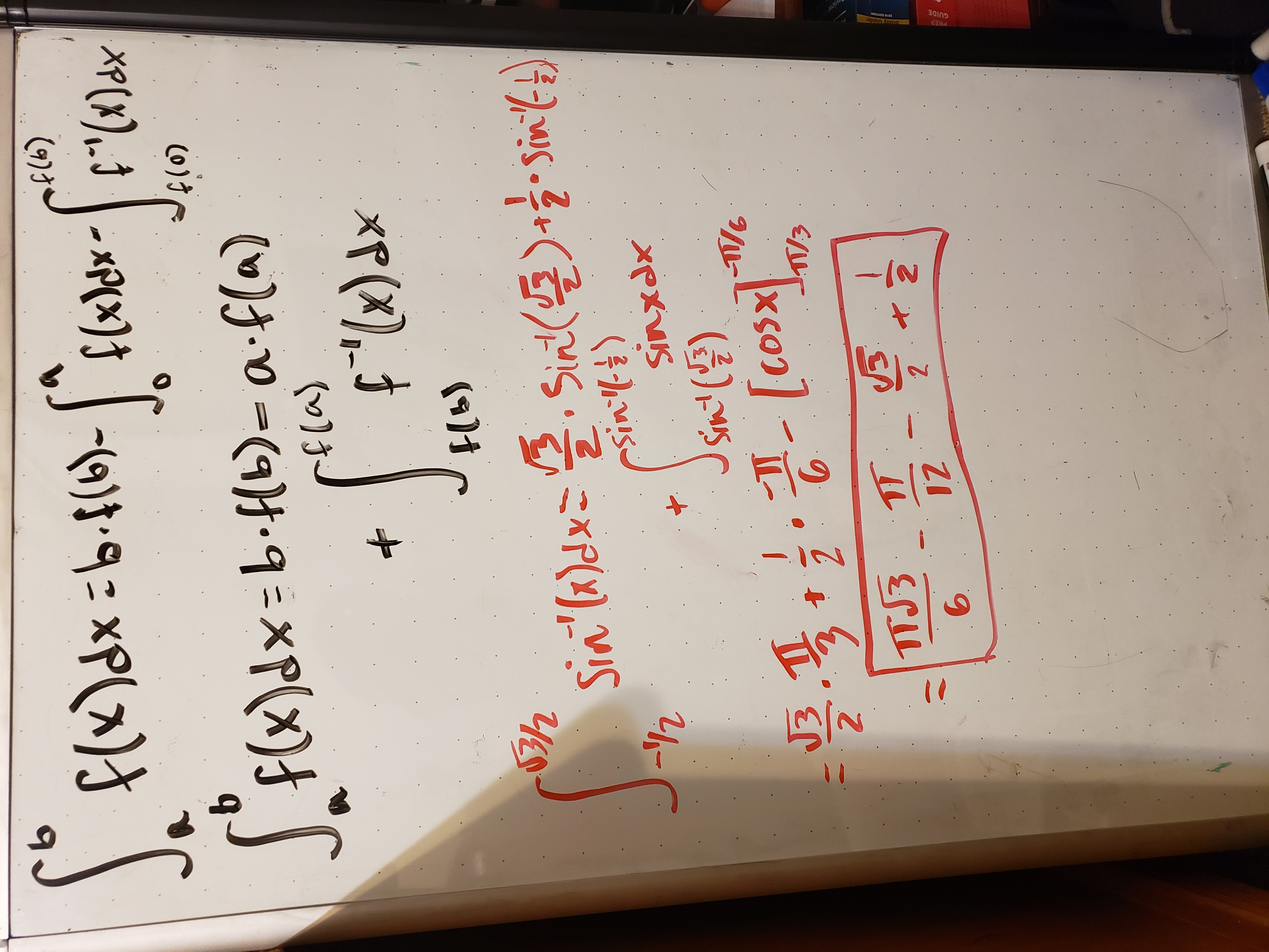
After putting what I’d found together into one formula I tested it out on the original inspiration for this endeavor. Using some clearly manufactured values, this seemed to work.
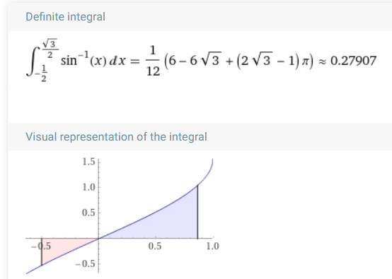
Using WolframAlpha we see this is accurate:
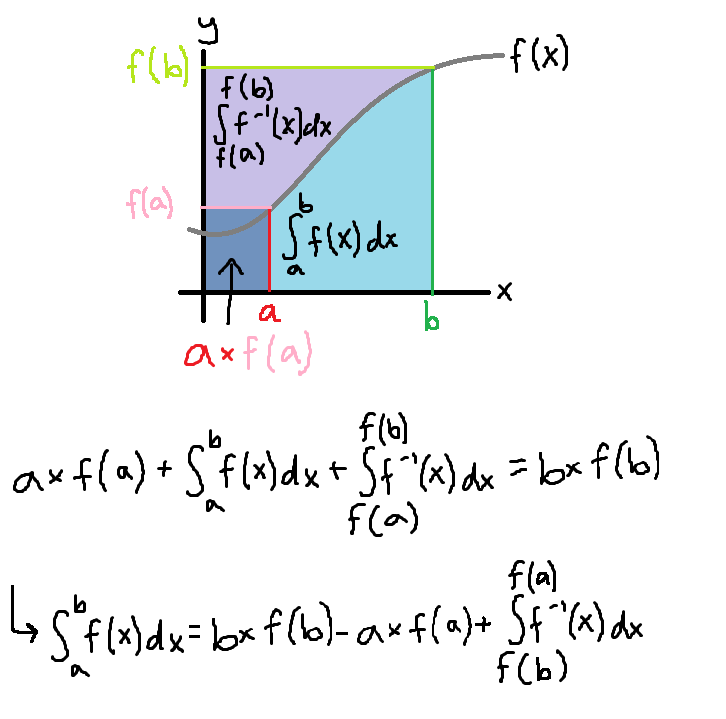
This diagram might provide a better idea of what is actually going on here. Note that this generic function is invertible on the interval from \(a\) to \(b\):
In truth, I haven’t really thought of this formula since this time, and it’s always felt a little “shaky” to me. I’m not quite sure how to explain the way I feel about it, but because of the nature of how I came up with this (very sloppily, not rigorously) I wouldn’t be surprised if someone is able to point out some flaw in my reasoning.
This being said, this formula has worked for the few carefully constructed examples I came up with at the time and no one has since shed light on any wrong thinking. One would definitely have to be careful to only use this for examples where both \(f\) and \(f^{-1}\) are defined throughout the entire range of the bounds from \(a\) to \(b\).
I show this formula to highlight how powerful a little bit of boredom and uninterrupted, unguided thought can be! In today’s culture and with today’s technology, there is always something to be doing or thinking about. Taking a break from moving quickly and letting our minds wander is something that we as humans have fallen out of touch with, and I truly believe this is among the biggest hinderances to solving a lot of problems that we face in the world today - not to mention the individual benfits that come from this regular intentional distancing.
For much of the recent years of my life, I’ve surrounded myself with lots of educational content (and trust me, there are tons of cool things to learn), but the true joy of this comes from taking these tools I’ve learned and discovering a new way to use them to solve a new problem. Many of the things you can find around this website came from many moments of raw pondering.
So take breaks! You never know what kind of things will come out of that powerful subconscious of yours!
Suliga Formula 2
Let’s kick it up a notch.
\[\int_{-\infty}^{\infty}e^{ax^{2}+bx+c} \space dx = \] \[\lim_{n \to \infty} e^{c - \frac{b^{2}}{4a}}\sqrt{\frac{\pi}{a}(e^{an} - 1)}\]
I first came up with this formula partway through my Junior year of high school. When Senior year came around and I wanted to secure my own parking spot in the crowded lot by giving it my own paint job, I decided to make it all math-related. I came up with a design that incorporated plenty of various mathematical formulas and figures, with the formula of my own to complete the design, which can be seen here lining the right side of the parking space.
Some other fun honorable mentions in this design include
- Euler’s formula and The Most Beautiful Equation in Math
- The gamma function and its connection to factorials
- The infamous \(-\frac{1}{12}\)

\[\int_{-\infty}^{\infty}e^{ax^{2}+bx+c} \space dx = \] \[\lim_{n \to \infty} e^{c - \frac{b^{2}}{4a}}\sqrt{\frac{\pi}{a}(e^{an} - 1)}\]
Sometimes when people see this daunting mess of symbols, I get asked
"So how does it work?" or "What does it do?"
These are valid questions given the very uninviting manner of the formula - there’s literally not any numbers anywhere. This can be be hard for many people to wrap their minds around what this means, but it’s actually very simple (given an exposure to integral calculus).
All this shows is that, if you’re going about your life and suddenly need to find \(\int_{-\infty}^{\infty}e^{-3x^{2}+7x-1} \space dx \), you’re in luck! By plugging \(-3, 7,\) and \(-1\) in for \(a, b,\) and \(c\) respectively, you’d know that the answer is exactly \(e^{\frac{37}{12}}\sqrt{\frac{\pi}{3}}\)! This is about \(22.34\).
This example paints a pretty accurate picture of how “useful” this formula is - basically zero. I’ve never had to use this for anything and I don’t expect to, however building up from a pretty useful example of this expression might shed some light on how it’s been used in the past heavily in forming modern statistics.
At this point, you probably think this is a meaningless idea to explore. However, one might notice that, when we plug in \(a = -1\), \(b = 0\), and \(c = 0\) to this formula, we can see that
\[\int_{-\infty}^{\infty}e^{-x^{2}} \space dx = \sqrt{\pi}\]
Whether you care at all about the initial formula or not, there’s no denying that this is pretty dang cool. We’re taking this weird infinite integral (whose integrand has no elementary antiderivative!) and getting \(\sqrt{\pi}\) out of it! We know that anywhere \(\pi\) shows it’s face, there’s a hidden circle to be found. In this instance, the circle is very hidden, but with a bit of thinking outside of the disc we can find it.
In fact, this example is where this discovery all began with Gauss in 1809. While understanding of ideas from This Video is not necessary just yet and will be explained in the extension below, it explains this particular example very well and will provide the best base for the information to come. This example has been titled as the Gaussian Integral.
Side Note: This video brushes over adding “\(\space rdrd\theta \space \)” when converting from a cartesian integral to an integral in polar form, which is the central step that makes this idea work at all. Even if you’re familiar with the Gaussian integral or multivariable calculus, I highly recommend watching at least This Short Video. It builds a very strong visual intuition for doing this when dealing with change-of-variable integration.
\[\int_{-\infty}^{\infty}e^{ax^{2}+bx+c} \space dx\]
Ok, so let’s start from the top and break this nasty integral down one piece at a time. We first notice that this integrand has no elementary antiderivative. What this means is that, using our normal operations \( + - \times \div \), exponentiation, trigonometric/hyperbolic function expression, their inverses, etc., we cannot construct the antiderivative.
For example, to evaluate \(\int_{a}^{b} 4x^{2} \space dx \), our first step is to find an antiderivative of \(4x^{2}\) - a function whose derivative is \(4x^{2}\). Using what many learn as the power rule, we know that this function takes the form of \(\frac{4}{3}x^{3}\), which I encourage you to check. The key point here is that, since we were able to come up with an explicity-defined antiderivative of \(4x^{2}\) using our normal notations, we can see that this function has an elementary derivative.
So going back to our problem, we’re stuck wondering where to go. We know that this integrand’s antiderivative is nonelementary because of this “\(x^{2}\)” term in the nasty exponent without any multiplied \(x\) term in the integrand. However, we were able to pull a trick (explained in the video) to convert this into a polar form and evaluate from there, but that only worked because we were integrating \(e\) raised to something squared.
This means that our first main step for evaluating this integral is to try to turn it into this form. We want to do some manipulations so that we have
\[\int_{-\infty}^{\infty} e^{f(x)^{2}} \space dx\]
Well, the first conflict to this idea is that we have this “\(\space + \space c \space\)” in our exponent. However, with some tricky algebra we can quickly remove this from the integral:
\[\int_{-\infty}^{\infty} e^{ax^{2}+bx+c} \space dx = \] \[\int_{-\infty}^{\infty} e^{ax^{2}+bx} \space e^{c} \space dx = \] \[e^{c} \int_{-\infty}^{\infty} e^{ax^{2}+bx} \space dx\]
Here we just used the fact that \(e^{c}\) is simply a constant, independent of \(x\), and so we can pull it ouside of the main integral.
At this point we can now use one of my favorite pieces of math to get this new integrand into the form that we want, Completing the Square.
\[e^{c} \int_{-\infty}^{\infty} e^{ax^{2}+bx} \space dx =\] \[e^{c} \int_{-\infty}^{\infty} e^{a(x^{2}+\frac{b}{a}x)} \space dx =\] \[e^{c} \int_{-\infty}^{\infty} e^{a(x^{2}+\frac{b}{a}x+\frac{b^{2}}{4a^{2}}-\frac{b^{2}}{4a^{2}})} \space dx =\] \[e^{c} \int_{-\infty}^{\infty} e^{a((x+\frac{b}{2a})^{2}-\frac{b^{2}}{4a^{2}})} \space dx =\] \[e^{c} \int_{-\infty}^{\infty} e^{a(x+\frac{b}{2a})^{2}-\frac{b^{2}}{4a}} \space dx =\] \[e^{c} \int_{-\infty}^{\infty} e^{a(x+\frac{b}{2a})^{2}} \space e^{-\frac{b^{2}}{4a}} \space dx =\] \[e^{c} \space e^{-\frac{b^{2}}{4a}} \int_{-\infty}^{\infty} e^{a(x+\frac{b}{2a})^{2}} \space dx =\] \[e^{c-\frac{b^{2}}{4a}} \int_{-\infty}^{\infty} e^{a(x+\frac{b}{2a})^{2}} \space dx\]
And look at that! We’ve reached a spot where we have the integral of \(e\) raised to something squared just like we wanted!
Now that was a lot that just happened, so lets first break down the steps we just took before we move on.
First, we factored out the \(a\) from our polynomial in the exponent. This is required in order to use completing the square. Then, we took our linear term of this polynomial, divided it by 2, and squared it. This step is the essence of the completing the square technique. At this point, we were able to see our perfect square arise, \(x^{2}+\frac{b}{a}x+\frac{b^{2}}{4a^{2}} = (x+\frac{b}{2a})^{2}\). We then distributed the \(a\) back into the expression.
Hopefully the last couple steps seem familiar to you, because it’s the same exact thing we did originally with the \(e^{c}\) term! In the same way, \(e^{-\frac{b^{2}}{4a}}\) is a constant independent of \(x\), so we can pull it out to the front of the integral. We can then combine the two terms into one exponent outside.
Our next step is to move this integrand (which still has a nonelementary antiderivative) into a polar representation in a tricky manner. For this step, we’re going to isolate our integral from the rest of the expression and tackle it individually. Let’s just call it \(I\) for integral (this is actually pretty standard when dealing with these kinds of problems funnily enough).
\[I := \int_{-\infty}^{\infty} e^{a(x+\frac{b}{2a})^{2}} \space dx\]
So in the context of our problem we can say
\[\int_{-\infty}^{\infty}e^{ax^{2}+bx+c} \space dx = Ie^{c-\frac{b^{2}}{4a}}\]
However, there’s a small amount of housekeeping to be done before diving into the Gaussian Integration step that will make things a lot easier for us. The following can be shown by a simple u-substitution:
\[I = \int_{-\infty}^{\infty} e^{a(x+\frac{b}{2a})^{2}} \space dx\] \[= \int_{-\infty}^{\infty} e^{au^{2}} \space du\]
There’s a cool way of thinking about this though that might get lost when working through the substitution. If we look at our integrand, we can see that, while we may not know what the graph of \(e^{ax^{2}}\) looks like, we do know it looks exactly the same as \(e^{a(x+\frac{b}{2a})^{2}}\), just shifted a bit left or right. In this expression, \(\frac{b}{2a}\) is what we call a phase shift as it is just shifting the original function somewhere else on the x-axis.
This is cool, but it doesn’t fully explain why these two expressions are equivalent when evaluated in the integral. The real reason we can do this is because of the fact that our bounds for integration are \(-\infty\) to \(\infty\). Think of this integral as sweeping through all of the number line, collecting all of the area between the x-axis and \(e^{a(x+\frac{b}{2a})^{2}}\). Because of this, we don’t have to care about any phase shift of \(e^{ax^{2}}\), since either way this area will be collected and accounted for in the infinite bounds of the integral. This is why we can say these two integrals are equal, if we had a definite integral, we wouldn’t be able to move any further.
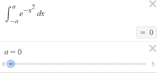
Side Note: Even given a definite integral, we could still get an extremely good approximation for our result, where the difference in estimated and actual values is negligible. For this to happen though, \(a\) must be less than \(0\) (more on this later) and the boundaries of integration must be far enough along the axes to collect the near total of area under the curve. As an example, look at \(e^{-x^{2}}\) below, and notice how the area under the curve barely changes as we spread out the bounds of integration once we get to the “flat part” of the graph. An important interjection, this graph will never fully touch the x-axis on either side, but we can see how quickly it becomes so close to this axis that it seems to be sitting directly on it. Also note what value it is approaching!

So at this point we have this \(I\) integral that we are trying to break down, and we just showed:
\[I = \int_{-\infty}^{\infty} e^{a(x+\frac{b}{2a})^{2}} \space dx\] \[= \int_{-\infty}^{\infty} e^{ax^{2}} \space dx\]
And now comes the power of Gauss’ Technique. Since \(x\) is an arbitrary variable, we can say both of these are equivalent:
\[I = \int_{-\infty}^{\infty} e^{ax^{2}} \space dx\] \[I = \int_{-\infty}^{\infty} e^{ay^{2}} \space dy\]
We can then multiply these two expressions to get the following:
\[I^{2} = \int_{-\infty}^{\infty} e^{ax^{2}} \space dx \int_{-\infty}^{\infty} e^{ay^{2}} \space dy\]
And since these two multiplied integrals don’t have any dependency conflicts (i.e. each integrand depends only on the variable being integrated over),
\[I^{2} = \int_{-\infty}^{\infty}\int_{-\infty}^{\infty} e^{ax^{2}} \space e^{ay^{2}} \space dxdy\] \[= \int_{-\infty}^{\infty}\int_{-\infty}^{\infty} e^{ax^{2} + ay^{2}} \space dxdy\] \[= \int_{-\infty}^{\infty}\int_{-\infty}^{\infty} e^{a(x^{2} + y^{2})} \space dxdy\]
And now comes the fun part - we see this \(x^{2} + y^{2}\) and think of polar coordinates. Using our definition of \(x^{2} + y^{2} = r^{2}\), we can change this integrand to \(e^{ar^{2}}\). But we also have to think about the rest of the integral, namely the bounds and the differentials.
Let’s start with the bounds. What we have now is \(x \in (-\infty, \infty)\), \(y \in (-\infty, \infty)\). When we think about these together, we can see that this range sweeps over all of \(\mathbb{R}^{2}\). This means that when we change to polar coordinates, we must find bounds for \(r, \theta\) that also sweep over all of \(\mathbb{R}^{2}\). There are actually infinite choices for this, but the easiest (and most standard) is \(r \in [0, \infty)\), \(\theta \in [0, 2\pi)\). Make sure you’re convinced that these bounds for \(r, \theta\) do in fact cover all of the \(\mathbb{R}^{2}\) plane. Think of \(\theta\) rotating once all the way around the origin with \(r\) extending from the origin all the way out to infinity. These two actions combined with one another will indeed collect all of \(\mathbb{R}^{2}\).
Now for the differentials. This portion will seem strange if you’ve never worked with change of variables in integration. Many of us may have been told to simply replace \(dxdy\) with \(rdrd\theta\) when changing to polar/spherical from cartesian like we’re doing here. I won’t explain here why we do this (Jacobians are wonderful and a great way to see this, but that’s just a lot more than you would need to know to grasp this idea, and was way above my head when I first came up with this formula), but as I mentioned before, This Video has a sufficient explanation.
So what have we figured out when changing our integral to a polar form? We know the bounds, integrand in polar coordinate notation, and differentials, which is all we need to build \(I\) back up.
\[I^{2} = \int_{-\infty}^{\infty}\int_{-\infty}^{\infty} e^{a(x^{2} + y^{2})} \space dxdy\] \[= \int_{0}^{2\pi}\int_{0}^{\infty} e^{ar^{2}} \space rdrd\theta\]
And we can split this double integral up into two independent multiplied integrals, similar to before:
\[I^{2} = \int_{0}^{2\pi} d\theta \int_{0}^{\infty} re^{ar^{2}} \space dr\]
And now, we can finally start actually integration as normal, since both of these integrands have elementary antiderivatives.
\[I^{2} = \int_{0}^{2\pi} d\theta \int_{0}^{\infty} re^{ar^{2}} \space dr\] \[= \Big[ \theta \Big] \Big|_{\theta = 0}^{2\pi} \Big[ \frac{e^{ar^{2}}}{2a} \Big] \Big|_{r = 0}^{\infty} \] \[= [ 2\pi ] \times \frac{1}{2a} [ e^{a\infty} - e^{0} ]\] \[= \lim_{n \to \infty} \frac{\pi}{a} ( e^{an} - 1 )\]
Let’s take a step back here. Here was that very hidden circle we were talking about - in order to find it we had to use 2 separate wacky integrals, multiply them, and then notice the polar form they took. This is such a cool way for pi to show up here. I like to think pi wakes up in the morning and then just goes around random unexpected places showing its face. And don’t even get me started on \(\pi^{2}…\)
But we’re not done just yet! We’ve just found
\[I^{2} = \lim_{n \to \infty} \frac{\pi}{a} ( e^{an} - 1 )\]
So it follows that
\[I = \lim_{n \to \infty} \sqrt{\frac{\pi}{a} ( e^{an} - 1 )}\]
And now, remembering how \(I\) was defined in the first place, we can put all of the pieces back together:
\[\int_{-\infty}^{\infty}e^{ax^{2}+bx+c} \space dx = Ie^{c-\frac{b^{2}}{4a}}\] \[= \lim_{n \to \infty} e^{c-\frac{b^{2}}{4a}} \sqrt{\frac{\pi}{a} ( e^{an} - 1 )}\]
\(\blacksquare\)
This looks like a lot, but there’s an important realization to be made here. Take a look at \(a\) in the formula. Firstly we’ll notice that this formula will not work altogether if \(a = 0\), and that’s because we have \(a\) in the denominator of two different fractions. But have no fear, if you come across an integrand of this type where there is no quadratic term, that’s incredibly simpler to solve that the one we just worked through.
Next, let’s consider what happens for other values of \(a\). I encourage you to think on this for a little - what do the graphs of \(e^{ax^{2} + bx + c}\) look like when \(a\) is positive? Negative?
Take a look at the diagram below. This is showing just \(e^{ax^{2}}\) for different values of \(a\), with \(a\) represented by the x-value of the point on the axis.

A fun little note: this gif happens to be 314 frames long :)
Hopefully from this animation you’re able to see where we’re going with this - whenever \(a\) is negative, the graph of the function looks like it hugs the x-axis with a little bump in the middle. In fact, no matter how small the magnitude, if \(a \lt 0\) this will be the case, and the area underneath this function is finite. However we see that, when \(a \gt 0\) the graph looks kind of parabolic, as it climbs up to infinity when approaching both \(\infty\) and \(-\infty\). Similarly to above, no matter how small the magnitude, if \(a\) is positive then the area underneath the graph will be infinite. These claims can also be verified algebraically very simply.
\[\int_{-\infty}^{\infty}e^{ax^{2}+bx+c} \space dx\]
What we can conclude from this when looking at our original problem above is that, this integral will be finite, or convergent, whenever \(a \lt 0\) and will have infinite value, called divergent, whenever \(a \gt 0\). We can actually simplify our formula a lot for the convergent case if we break this apart under a new assumption.
For this section we will assume \(a \lt 0\), meaning the graph of \(e^{ax^{2}+bx+c}\) “hugs” the x-axis. Let’s take a look at our conclusion and see what we can break down under this assumption:
\[\int_{-\infty}^{\infty}e^{ax^{2}+bx+c} \space dx = \] \[\lim_{n \to \infty} e^{c - \frac{b^{2}}{4a}}\sqrt{\frac{\pi}{a}(e^{an} - 1)}\]
The first place that \(a\) shows up here is in this fraction in the exponent. There’s actually nothing that can be simplified here, so let’s move on to the next place \(a\) is found. This fraction in the square root also can’t be simplified further, but something interesting can be seen in this next section - when we have \(\lim_{n \to \infty} \space e^{an}\), we now know this is just \(0\) with our information about \(a\).
This is because \(\lim_{n \to \infty} \space e^{an}\) is essentially \(e^{-\infty}\) which is the same as \(\frac{1}{e^{\infty}}\). \(1\) divided by a really big number yields a number very small in magnitude, and taking this to the infinite case will yield exactly \(0\).
This means that \(\lim_{n \to \infty} \sqrt{\frac{\pi}{a}(e^{an} - 1)} \) just becomes \(\sqrt{-\frac{\pi}{a}}\). Remember that \(a\) is negative here, so that minus sign will cancel with the negative value of \(a\), so don’t worry about any complex business. To show this, we could even make this into \(\sqrt{\frac{\pi}{|a|}}\).
So under the assumption \(a \lt 0\), we now have this expression:
\[\int_{-\infty}^{\infty}e^{ax^{2}+bx+c} \space dx = e^{c - \frac{b^{2}}{4a}}\sqrt{\frac{\pi}{|a|}}\]
Isn’t that much cleaner?